Texas A&M UniversityFall 2026

Mathematics for
Visual Computing

See the geometry. Build the computation. Use mathematics to understand how visual data is represented, transformed, projected, analyzed, and learned.

15
connected weeks
5
hands-on assignments
0
written exams
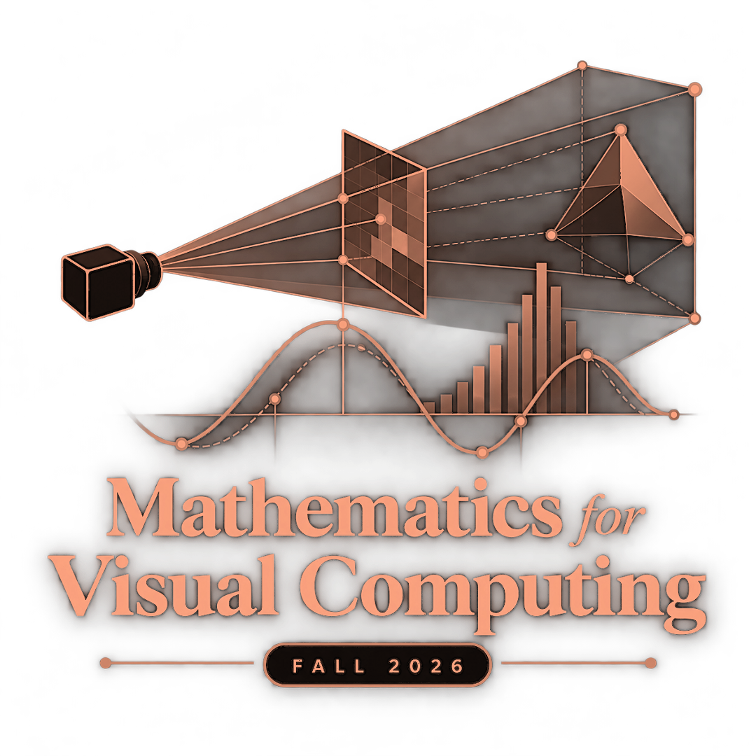
Course emblem combining a geometric surface, coordinate axes, a transformation matrix, and the course title A = UΣVᵀ x′ = Rx + t λx = K[R|t]X
Begin with intuition

Course philosophy

Rigorous mathematics,
made visually meaningful.

The course develops mathematical intuition and computational skill through theory, hands-on exercises, and programming projects in visualization, graphics, computer vision, and computational media.

The organizing principle
Understand what a mathematical object does before treating it as a formula to memorize.

Vectors become directions and measurements. Matrices become transformations. Subspaces become models. Cameras become projective maps. Fourier coefficients become visual frequencies. Neural layers become affine maps followed by nonlinearities.

CourseVIZA 689/601
Credits3
InstructorSuryansh Kumar
PrerequisitesMATH 152 and VIST 272, or permission
FormatApplication-driven lectures, exercises, and projects

What you will be able to do

Five capabilities that accumulate across the semester

01

Transform visual data

Apply vectors, matrices, eigenanalysis, SVD, and projections to visual-computing problems.

02

Model rotation

Use complex numbers and quaternions to represent 2D and 3D orientation.

03

Reason in frequency

Use Fourier transforms to analyze and manipulate visual signals and images.

04

Interpret neural models

Understand neural networks as structured function approximators built from linear algebra.

05

Build applications

Program advanced mathematical ideas and turn them into working visual demonstrations.

The learning arc

One continuous progression,
not fifteen disconnected topics.

Each phase provides the language needed by the next: algebra supports geometry, geometry supports cameras, cameras create data, and data motivates signal and neural representations.

01

Weeks 1–3

Build the language of linear algebra

Move from vectors and matrices to linear systems, subspaces, rank, basis, and dimension.

Enter Foundations
02

Weeks 4–6

Understand structure and transformation

Study rigid motion, invertibility, eigenstructure, and singular-value decomposition.

Enter Geometry
03

Weeks 7–10

Fit, reduce, project, and calibrate

Connect least squares and PCA to image transformations, camera models, and calibration.

Enter Data & Projection
04

Weeks 11–13

Represent rotation and visual signals

Use complex numbers, quaternions, and Fourier analysis to model motion and imagery.

Enter Representations
05

Weeks 14–15

From linear maps to visual intelligence

Interpret multilayer perceptrons through linear algebra and synthesize the complete course pipeline.

Enter Learning & Synthesis
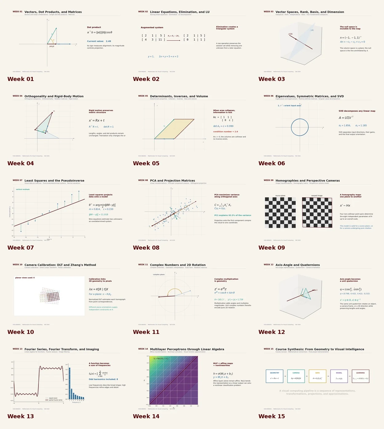
View the complete visual mapAll 15 weekly concept visuals at a glance
Contact sheet showing the mathematical visualization for each of the fifteen course weeks

Weekly material

Follow the mathematics
from vectors to visual intelligence.

Every week combines the syllabus topics, a concise conceptual explanation, key equations, a visual-computing connection, and a mathematically generated concept video.

Showing all 15 weeks

Mathematical concept visual

Linear combination, vector projection, and the action of a matrix on a grid.

Foundations

Week 1 · Intro to Linear Algebra for Visual Computing—I

Vectors, Dot Products & Matrices

Begin with the objects that carry visual information: vectors encode coordinates, directions, colors, and features, while matrices organize and transform them.

Syllabus focus

  • Vectors and linear combinations
  • Length and dot products
  • Matrices

Core idea

A linear combination builds a new vector from existing directions. The dot product measures alignment and produces projections. A matrix is best understood through the transformation it applies.

v = αa + βbaᵀb = ‖a‖‖b‖ cos θy = Ax

Visual computing connection. These ideas appear immediately in coordinate changes, feature similarity, surface normals, color transforms, and geometric modeling.

Open the Week 1 visual
Mathematical concept visual

An exact two-equation system, row elimination, and a verified LU factorization.

Foundations Assignment 1

Week 2 · Intro to Linear Algebra for Visual Computing—I

Linear Equations, Elimination & LU

Turn collections of constraints into solvable systems, then expose the triangular structure that makes repeated solution efficient.

Syllabus focus

  • Solving linear equations
  • The idea of elimination
  • LU decomposition

Core idea

Elimination replaces a system by an equivalent triangular one. LU decomposition records the elimination process as a product of lower- and upper-triangular matrices.

Ax = bA = LULy = b; Ux = y

Visual computing connection. Linear systems arise in reconstruction, interpolation, image processing, geometry, and the estimation of model parameters.

Open the Week 2 visual
Mathematical concept visual

A rank-two column space, a dependent column, and a null-space direction mapped to zero.

Foundations

Week 3 · Vector Spaces and Subspaces

Vector Spaces, Rank, Basis & Dimension

Move beyond individual vectors to the spaces they span, and learn how rank and null spaces reveal information, redundancy, and ambiguity.

Syllabus focus

  • Spaces and subspaces of vectors
  • Rank
  • Independence, basis, and dimension
  • The four fundamental subspaces

Core idea

A basis gives a minimal coordinate system for a space. Rank counts independent directions captured by a matrix; the null space contains directions that the matrix cannot observe.

rank(A) + nullity(A) = nAx = 0col(A) = span{a₁,…,aₙ}

Visual computing connection. Rank explains degeneracy in data, low-dimensional structure in images and shapes, and unobservable directions in inverse problems.

Open the Week 3 visual
Mathematical concept visual

A shape undergoing rotation and translation while lengths, angles, and dot products remain unchanged.

Geometry Assignment 2

Week 4 · Orthogonality and Rigid Body Motion

Orthogonality & Rigid-Body Motion

Use orthogonality to create stable coordinates and rotation matrices that preserve the metric structure of a visual scene.

Syllabus focus

  • Orthogonality of subspaces
  • Orthonormality and rotation matrices
  • Rigid-body motion

Core idea

Orthonormal bases preserve lengths and angles. A proper rotation satisfies RᵀR = I and det(R) = 1; translation then completes a rigid-body transformation.

RᵀR = Idet(R) = 1x′ = Rx + t

Visual computing connection. Rigid transforms are the basic language of camera pose, object motion, registration, robotics, and 3D graphics.

Open the Week 4 visual
Mathematical concept visual

Area scaling under a linear map and the approach to singularity as a parallelogram collapses.

Geometry

Week 5 · Determinants and Inverses

Determinants, Inverses & Volume

Connect algebraic invertibility to a geometric question: does a transformation preserve information or collapse space?

Syllabus focus

  • Determinant properties
  • Permutations and cofactors
  • Inverses and volumes

Core idea

The determinant measures signed area or volume scaling. A zero determinant means the transformation collapses at least one dimension and therefore has no inverse.

area(AΩ) = |det A| area(Ω)A⁻¹A = Idet(A) = 0 ⇒ singular

Visual computing connection. Invertibility matters in image warping, coordinate recovery, numerical stability, and the detection of degenerate configurations.

Open the Week 5 visual
Mathematical concept visual

A unit circle mapped to an ellipse, orthogonal eigendirections, and the rotate–scale–rotate stages of SVD.

Geometry Assignment 3

Week 6 · Eigen Values and Eigen Vectors

Eigenvalues, Symmetric Matrices & SVD

Find the directions a transformation treats specially, then decompose any linear map into orthogonal rotations and axis-aligned scaling.

Syllabus focus

  • Eigenvalues and eigenvectors
  • Symmetric and positive-definite matrices
  • Singular value decomposition

Core idea

An eigenvector keeps its direction under a matrix. For symmetric matrices, eigenvectors can be chosen orthonormal. SVD extends this geometric decomposition to any matrix.

Av = λvA = QΛQᵀA = UΣVᵀ

Visual computing connection. Eigenanalysis and SVD support compression, denoising, conditioning, PCA, low-rank models, and many vision algorithms.

Open the Week 6 visual
Mathematical concept visual

An overdetermined line fit with vertical residuals, the normal-equation condition, and the pseudoinverse solution.

Data & Projection

Week 7 · Least Squares and Pseudo Inverses

Least Squares & the Pseudoinverse

When noisy visual measurements do not satisfy a model exactly, estimate the parameters whose prediction is closest to the data.

Syllabus focus

  • Visual data modeled as matrices
  • Underdetermined and overdetermined systems
  • Least squares and normal equations

Core idea

Least squares projects the observation onto the model subspace. At the optimum, the residual is orthogonal to every column of the design matrix.

x* = arg minₓ ‖Ax − b‖²Aᵀ(Ax* − b) = 0x* = A⁺b

Visual computing connection. This is the backbone of line fitting, calibration, triangulation, motion estimation, and many inverse problems.

Open the Week 7 visual
Mathematical concept visual

A correlated point cloud, its principal axes, and projection onto the dominant component.

Data & Projection Assignment 4

Week 8 · Visual Computing Application—I

PCA & Projection Matrices

Use projection to retain the most informative directions in high-dimensional visual data while discarding redundancy.

Syllabus focus

  • Matrices and linear transformations
  • Principal component analysis
  • Projection matrices and applications

Core idea

PCA centers the data, finds covariance eigendirections, and projects onto the directions of largest variance. An orthogonal projector is symmetric and idempotent.

C = (1/n)XᵀXP = UUᵀx̂ = μ + U Uᵀ(x − μ)

Visual computing connection. PCA provides compact models of appearance, shape, motion, and features, and clarifies the geometry of dimensionality reduction.

Open the Week 8 visual
Mathematical concept visual

A true projective warp, a checkerboard homography, and the pinhole perspective relationship.

Data & Projection

Week 9 · Visual Computing Application—II

Image Transformations, Homographies & Cameras

Connect coordinates in images to projective geometry and understand how a camera converts a 3D scene into a 2D measurement.

Syllabus focus

  • Image transformation
  • Homography matrix
  • Modeling a perspective camera

Core idea

A homography is a projective transformation of a plane. Perspective projection divides by depth, so farther points appear smaller in the image.

x′ ∼ Hxx = fX/Zλx = K[R | t]X

Visual computing connection. These models drive image rectification, mosaicing, planar tracking, augmented reality, and 3D-to-2D projection.

Open the Week 9 visual
Mathematical concept visual

Normalized DLT for planar homographies followed by Zhang constraints that recover camera intrinsics.

Data & Projection Project Proposal

Week 10 · Visual Computing Application—III

Camera Calibration: DLT & Zhang’s Method

Estimate the parameters that connect rays in a camera to pixel coordinates, using correspondences and multiple views of a planar pattern.

Syllabus focus

  • Camera calibration
  • Direct Linear Transform (DLT)
  • Zhang’s approach

Core idea

DLT estimates a projective mapping from linear constraints. Zhang’s method combines planar homographies from different orientations to recover the intrinsic calibration matrix.

x ∼ PXP = K[R | t]h₁ᵀK⁻ᵀK⁻¹h₂ = 0

Visual computing connection. Calibration is required whenever metric geometry, accurate pose, measurement, or multi-view reconstruction is expected from images.

Open the Week 10 visual
Mathematical concept visual

A point rotating on the complex plane with constant modulus and its equivalent 2D rotation matrix.

Representations

Week 11 · Understanding Rotation in 2D and 3D—I

Complex Numbers & 2D Rotation

Represent a 2D point as a complex number and turn rotation into multiplication by a unit-magnitude complex number.

Syllabus focus

  • Complex-number operations
  • Geometric interpretation
  • Euler form and rotation-matrix representation

Core idea

Euler’s formula joins trigonometry and complex exponentials. Multiplication by eⁱᶿ rotates a point by θ without changing its magnitude.

eⁱᶿ = cos θ + i sin θz′ = eⁱᶿzR(θ) = [[cosθ, −sinθ],[sinθ, cosθ]]

Visual computing connection. Complex arithmetic gives a compact language for 2D rotations, periodic motion, phasors, and frequency-domain representations.

Open the Week 11 visual
Mathematical concept visual

An arbitrary 3D axis, Rodrigues rotation, and the equivalent unit-quaternion action on a vector.

Representations Assignment 5

Week 12 · Understanding Rotation in 2D and 3D—II

Axis–Angle, Quaternions & Camera Rotation

Represent 3D orientation using a rotation axis and angle, then encode the same rotation compactly with a unit quaternion.

Syllabus focus

  • Axis–angle representation
  • Quaternions
  • Application to camera modeling

Core idea

Axis–angle expresses a rotation geometrically. The corresponding unit quaternion uses half the rotation angle and composes rotations through quaternion multiplication.

q = (cos(θ/2), û sin(θ/2))v′ = q v q⁻¹R = exp(θ[û]×)

Visual computing connection. Quaternions are widely used for camera orientation, smooth interpolation, animation, and robot motion without coordinate singularities.

Open the Week 12 visual
Mathematical concept visual

A square-wave Fourier series built from odd harmonics and a genuine 2D FFT low-pass image reconstruction.

Representations

Week 13 · Visual Computing Application—IV

Fourier Series, Fourier Transform & Imaging

Treat functions as combinations of basis functions and reveal how visual signals distribute their energy across frequencies.

Syllabus focus

  • Linear algebra for functions
  • Fourier series and Fourier transform
  • Applications to imaging

Core idea

Fourier analysis represents a signal as a weighted sum of sinusoids or complex exponentials. Frequency coefficients separate broad structure from fine detail.

f(x) = Σₖ cₖeⁱᵏˣF(u,v) = 𝓕{f(x,y)}f = 𝓕⁻¹{F}

Visual computing connection. The frequency domain explains filtering, denoising, sharpening, sampling, compression, and image reconstruction.

Open the Week 13 visual
Mathematical concept visual

An exact two-unit ReLU construction for XOR and the piecewise-linear regions created by affine maps plus activation.

Learning & Synthesis

Week 14 · Multi-layer Perceptron (MLP)

Multilayer Perceptrons Through Linear Algebra

See a neural network as a sequence of affine maps and nonlinearities that bends input space into a useful representation.

Syllabus focus

  • MLPs through the lens of linear algebra
  • Affine transformation and nonlinear activation
  • Applications to visual computing

Core idea

Each layer applies a matrix transformation and bias, followed by a nonlinear activation. Without the nonlinearity, many layers collapse into a single affine map.

h = σ(Wx + b)f(x) = W₂σ(W₁x + b₁) + b₂ReLU(z) = max(0,z)

Visual computing connection. This viewpoint links classical linear algebra to learned visual representations, implicit functions, and nonlinear approximation.

Open the Week 14 visual
Mathematical concept visual

A course-wide pipeline linking geometry, projection, low-rank models, Fourier representations, and neural approximation.

Learning & Synthesis Final Project

Week 15 · Course Revision; Final Project Presentation and Demo

Course Synthesis & Final Project

Bring the semester together as a connected visual-computing pipeline rather than a collection of isolated formulas.

Syllabus focus

  • Course revision
  • Final project presentation
  • Visual demo and synthesis

Core idea

Geometry represents the scene; cameras project it; matrix models organize data; signal bases expose structure; neural functions approximate complex visual relationships.

geometry → camera → data → signal → learningx′ = Rx+tλx = K[R|t]Xh = σ(Wx+b)

Visual computing connection. The final project demonstrates how mathematical representation, computation, and visual reasoning work together in a complete application.

Open the Week 15 visual

Assessment

Demonstrate understanding
by making mathematics work.

There are no written examinations. Evaluation centers on assignments, a final project, participation, and the ability to demonstrate authentic work.

100%practice, projects
& participation
60%

Five assignments

Programming and concept work connected to material discussed in class.

35%

Final project

Teams of two or three are strongly encouraged, with a final presentation and visual demonstration.

5%

Participation

Attendance, in-class activity, timely work, final presentation participation, and a demo video clip.

Project-centered: the final exam period may be used for final project presentations.

Authentic work: students should retain records and be able to explain and demonstrate submitted work.

Schedule: weekly topics and timing may adjust in response to class interaction.

Resources & course information

Everything needed
to begin the course.

Course access

Start with the official syllabus

The syllabus contains complete course policies, grading details, learning outcomes, recommended resources, and university statements.

Download syllabus

Computing

Required setup

  • A serviceable laptop computer
  • MATLAB through the Texas A&M academic license
  • Python, NumPy, SciPy, and Matplotlib as useful computational resources

Recommended references

Books supporting the course

  • Gilbert Strang, Introduction to Linear Algebra, 6th ed.
  • John Vince, Mathematics for Computer Graphics, 5th ed.
  • John Vince, Quaternions for Computer Graphics
  • Marschner & Shirley, Fundamentals of Computer Graphics, 4th ed.